Vectors and Matrix Operations
We introduced how to manipulate vectors and matrices in NumPy. When we use SymPy we can do this symbolically.
Ex 4.3.1 Defining a vector
# Ex 4.3.1
import sympy as smp
smp.init_printing()
u1,u2,u3=smp.symbols('u1 u2 u3 ')
u=smp.Matrix([u1,u2,u3])
u
Ex 4.3.2 Addition and Multiplication
# Ex 4.3.2
import sympy as smp
smp.init_printing()
u1,u2,u3,v1,v2,v3=smp.symbols('u1 u2 u3 v1 v2 v3')
u=smp.Matrix([u1,u2,u3])
v=smp.Matrix([v1,v2,v3])
2*(u+v)
Ex 4.3.3 Dot Product
If u and v are vectors, then the dot product is u.dot(v)
# Ex 4.3.3
import sympy as smp
smp.init_printing()
u1,u2,u3,v1,v2,v3=smp.symbols('u1 u2 u3 v1 v2 v3')
u=smp.Matrix([u1,u2,u3])
v=smp.Matrix([v1,v2,v3])
u.dot(v)
Ex 4.3.4 Cross Product
If u and v are vectors, then the cross product is u.cross(v)
# Ex 4.1.20
import sympy as smp
smp.init_printing()
u1,u2,u3,v1,v2,v3=smp.symbols('u1 u2 u3 v1 v2 v3')
u=smp.Matrix([u1,u2,u3])
v=smp.Matrix([v1,v2,v3])
u.cross(v)
Ex 4.3.5 Norm
# Ex 4.3.5
import sympy as smp
smp.init_printing()
u1,u2,u3=smp.symbols('u1 u2 u3')
u=smp.Matrix([u1,u2,u3])
u.norm()
4.3.6 Projections
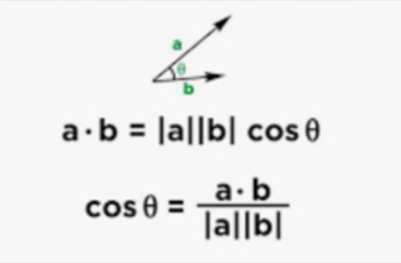
 Consider two vectors a and b. The length of the projection of b on a is given by |b|cos𝛉. As a vector, this projection has a direction given by a unit vector in the direction of a.
In this problem we will define two vectors u and v and find the projection of u on v. The projection is $|u|\cos(\theta)$ times a unit vector in the direction of v. $|\overrightarrow{u}|\cos(\theta)\frac{\overrightarrow{v}}{|\overrightarrow{v}|}=|\overrightarrow{u}|\frac{\overrightarrow{v}\cdot \overrightarrow{v}}{|\overrightarrow{u}||\overrightarrow{v}|}\frac{\overrightarrow{v}}{|\overrightarrow{v}|}=\frac{\overrightarrow{u}\cdot \overrightarrow{v}}{|\overrightarrow{v}|^2}\overrightarrow{v}$
# Ex 4.3.6
import sympy as smp
smp.init_printing()
u1,u2,u3,v1,v2,v3=smp.symbols('u1 u2 u3 v1 v2 v3')
u=smp.Matrix([u1,u2,u3])
v=smp.Matrix([v1,v2,v3])
(u.dot(v)/(v.norm())**2)*v
Ex 4.3.7 Lines and Planes in 3-space
$\overrightarrow{r}=\overrightarrow{r_0}+t\overrightarrow{v}$ This defines a parametric line in space where t is a parameter.
# Ex 4.3.7
import sympy as smp
smp.init_printing()
r0,v,t=smp.symbols('r0 v t')
r0=smp.Matrix([1,1,1])
v=smp.Matrix([1,3,-1])
r=r0+t*v
r
Graphing with Sympy:
References: \ https://sympy-plot-backends.readthedocs.io/en/latest/overview.html \ https://www.cfm.brown.edu/people/dobrush/am33/SymPy/part1.html \ https://www.youtube.com/watch?v=gm0ZlVpfmmo \ In the next example we rerun the last example, but include a plot. Note: the x,y, and z coordinates are the indexed values of the vector r.
4.3.8 Graphing a Parametric Representation of a Straight Line
lines 8-12 define the parametric line with parameter t and direction given by vector v. The line passes through r0 and vector v has components of [1,3,1]. Note this is not a unit vector.
lines 15-17 The x,y and z coordinates of any point on the line is given by the 0th, 1st, and second component of the r vector.
line 19 This is the SymPy plotting routine for a 3d parametric plot. The coordinates x,y,z were previously defined, and the tuple (t,0,5) specifies the linear range of values of the parameter t.
# Ex 4.3.8
import sympy as smp
from sympy.plotting import plot3d_parametric_line
smp.init_printing()
r0,v,t,x,y,z=smp.symbols('r0 v t x y z')

# a point on the line and the vector defining the direction of the line
r0=smp.Matrix([0,0,0])
v=smp.Matrix([1,3,1])

# the vector r to plot with the parameter t
r=r0+t*v

# x,y,z are the 0th,1st and 2nd component of vector r.
x=r[0]
y=r[1]
z=r[2]

plot3d_parametric_line(x,y,z,(t, 0, 5),xlabel='x',ylabel='y',zlabel='z')
Ex 4.3.9 Graphing x=cos(u), y=sin(u), z=(u,-5,5)
In this example, the parameter of the curve is u. In line 5 we specify the plot giving x and y as trig functions (remember you must use smp.sin and smp.cos. The z axis is linear with (u,-5,5). This is a 3D Lissajous figure.
# Ex 4.3.9
import sympy as smp
from sympy.plotting import plot3d_parametric_line
smp.init_printing()
u=smp.symbols('u')
plot3d_parametric_line(smp.cos(u), smp.sin(u), u, (u, -5, 5),xlabel='x',ylabel='y',zlabel='z')
Ex 4.3.10 Equation for a plane
Suppose we have a point $P_0$ and we consider all <x,y,z> values such that the vectors from $P_0$ to <x,y,z> satisfy the condition that $\overrightarrow v$ are normal to a vector $\overrightarrow n$.( NOTE the normal vector does not have to be a unit normal.) The plane is then defined by $ \overrightarrow n \cdot (P_0)-<x,y,z>)=0$
Lines 7-9r is the set of all points in the plane; P0 is a point in the plane; n is a normal to the plane.
Line12 The equation of the plane is defined by n.dot(P0-r)=0. res is the solution of this equation for z.
Line 12 res will be a list of all solutions; there is only one solution, but we must get that expression using res[0]
Line 18 here we plot z (res[0] vs x and y where x & y take on values between -5 and 5.
# Ex 4.3.10
import sympy as smp
from sympy.plotting import plot3d
smp.init_printing
x,y,z=smp.symbols('x y z')

# We want to find all points  r=<x,y,z> passing thru P0 <4,4,8> which is normal to vector <1,1,1>
r=smp.Matrix([x,y,z])
P0=smp.Matrix([4,4,8])
n=smp.Matrix([1,1,1])

# Here we take the function n.dot(P0-r)=0 and solve for z
res=smp.solve(n.dot(P0-r),z)

# res is a list with one element, but we must take the value of that element res[0].  This is the value of z
print(' Equation of the Plane:  z=',res[0])

# plot the expression res[0] as x and y range from -5 to 5
plot3d(res[0],(x,-5,5),(y,-5,5))